Anatomy of a Particle Physics Experiment
Recently I returned from a particle physics experiment at the Paul Scherrer Institut, a nuclear research lab in Switzerland. I was one of ten students from the University of Heidelberg and ETH, Zürich who had two weeks of (nearly) free reign to carry out an experiment on the PSI’s proton beam line. To put into perspective how crazy that is, ordinarily the going rate for such a privilege is €10,000s per day!
Our goal was to measure a mysterious number called the “Panofsky ratio”. The ratio is named after Wolfgang Panofsky, first to attempt to measure it, and corresponds is the relative likelihood of two events involving particles called protons and pions occurring. It is important, because historically its value strongly contradicted the expectation of theoretical physicists.
The two processes occur by means of two different forces—one by the weak interaction and the other by quantum electrodynamics—and so the ratio was expected to be somewhere near the ratio of strengths of these interactions, give or take a few corrections, which happens to be around 30 (\(\gamma\)s represent photons):
\begin{equation} \text{Panofsky Ratio } P = \frac{R(p\pi\rightarrow n^* \rightarrow \gamma \gamma)}{R(p \pi \rightarrow n \gamma)} \label{eq:pr} \end{equation}
However, when Panofsky measured the ratio, he got a value of around 0.8. Notwithstanding the fact that this is actually wrong, it’s far enough enough from 30 to prove there is more going on than was expected. Panofsky’s measurement is off by about half from the true value of 1.546±0.009;1 initially we scoffed that such an eminent scientist could get a measurement so wrong. Well, having all but completed the analysis, how my view has changed! This is not an easy measurement to get right.
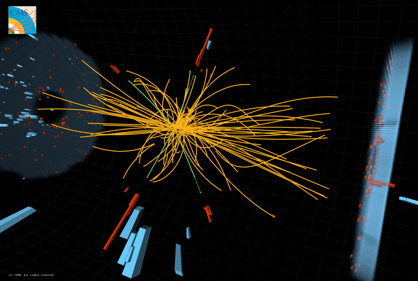
Higgs candidate event from LHC. All of the tracks are particles emanating out from the collision point. The tracks are curved because, usefully, charged particles (such as electrons and protons) are deflect according to their mass and charge when they pass through a magnetic field. The red and blue blocks show how much energy was deposited in the calorimeter at that point. There are perhaps seven or eight independent events here, but only one is a Higgs event. Taken from CERN.
Particle Physics: The Basic Principle
In line with almost all particle physics experiments, the measurement of the ratio was essentially a counting experiment. You essentially fire particles at a target, be that a stationary target as here, or an opposite-travelling beam as with the LHC, and try to detect the off-coming particles so you can reconstruct what processes happened.
With reporting on the news about the discovery of the Higgs boson, anyone could be forgiven for thinking, well, if you fire the right projectile at the right target, and watch and wait, eventually you’ll find what you’re looking for.
Of course, nothing is ever quite so simple. Take the LHC. On the right is what an LHC Higgs boson event really looks like. In reality, reconstructed events like this are primarily for show – the actual analysis of these things is all done by specialized software (and hardware?) – indeed, it was one of my responsibilities to co-write this software for our group.
Actually, the real challenge, not just in ours, but in all particle physics experiments, comes from the fact that interesting events hardly ever occur–it’s rather like searching for a silver needle amidst a stack of silvery grey ones. It’s a stack of needles because, as a necessary artefact of the triggering mechanism described below, most of the events really look very similar; only careful offline analysis can sift out the silver.

Detecting interesting events is rather like searching for a silver needle in a massive stack of silvery-grey ones.
The other main difficulty in the Panofsky ratio measurement is that all of the detectable particles are electrically neutral, not charged, particles. Neutral particles are harder to detect, track, and measure accurately than are charged particles. To measure charged particles, you just stick them in a magnetic field and measure the curvature of their paths; they can literally be observed with the naked eye (as seen in cloud chambers). Neutral particles, however, just pass right through, invisible.
To measure neutral particles, all you can do is hope they will get stuck in your detector and dump all their energy there, that way you can read their energy off; although with more advanced tracking systems, you can actually reconstruct their trajectories and velocities to identify them more precisely. Our set-up was much more modest, but we knew exactly which particles to expect at exactly which energies, so particle identification was already done in the energy measurement.
Data Acquisition
In order to record the data from the experiment, some kind of data acquisition system is needed. For larger experiments, there can be literally millions of read-out channels, all of which must be accessed and their data read off and stored for each interesting event. Because of the extremely high rate of background events (thousands per second in this case), it is neither technologically possible nor desirable to record all of this data.
For example, we had access to seven 8-bit ADCs (Analogue-to-Digital Converter) which ran at 200MHz to read off data–that’s a data throughput rate in the region of 1½ GB/s! Clearly even we had to whittle this down somehow, but for larger experiments this aspect of the experiment is critical. The usual trick is to employ a triggering mechanism to wake the electronics up when something interesting (might have) happened.
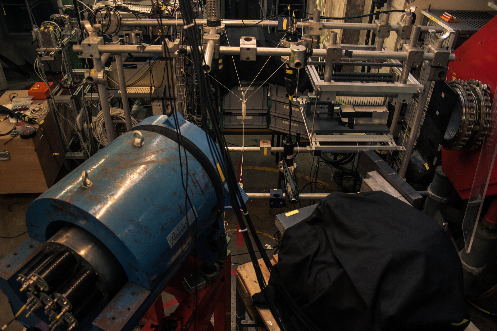
Experimental set-up. The black paddles are the scintillators used to notify the electronics when a particle has passed through them. You can also see the lead and plastic shielding for the calorimeters (hidden under black cloth) poking into the picture on the right, to reduce the background stream of particles directly from the beam pipe or interactions with the metal frame etc. The target is suspended in the plastic bag at the centre of the set-up.
To actually implement a triggering mechanism, we made use of scintillators, the long black paddles covered in tape. Scintillators work by giving out a signal when a particle passes through; if two or more are properly aligned in time, this allows the use of simple electronics to detect co-incident signals etc. which can tell you immediately something about how interesting the event is, and therefore whether you want to store and analyze it.
How Are particles’ energies measured?
The actual energy measurement, the most important part of the whole endeavour, comes from the calorimeters. We used two different calorimeter types, one of BGO (bismuth germanate) and the other NaI (sodium iodide).2 Calorimeters measure energy by attempting to stop the particle which is entering, and sending signals about the electric charge inside to the electronics and data acquisition system. The signals are taken over a specific time interval, which creates an event trace showing how the voltage changed over a few nanoseconds. The area under the signal trace is related to how much energy the incident particle had, hopefully linearly.3
I’ll upload an example event trace if I can get my hands on one.
The Panofsky Ratio
Ultimately, we were seeking a spectrum looking something along the lines of the spectrum on the left. The spectrum is a histogram of the area under the signal traces from the calorimeters. From the calorimeters, we obtained energy histograms such as on the right:
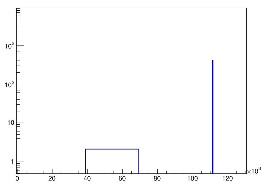
The ideal spectrum. The form of this spectrum is the goal, although such sharp peaks would obviously be smeared into Gaussian peaks etc. The Panofsky ratio is obtained by taking the ratio of events in the oblong to those in the peak. The x-axis scale is arbitrary.
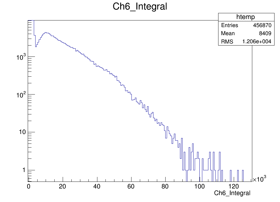
This is the raw output of the large blue sodium iodide calorimeter. It doesn’t particularly resemble the ideal plot. Hopefully it will look a bit better after background subtraction.
Obviously, there is an absolute ton of background which needs to be dealt with!
Removing Background and Recovering the Ideal Plot
Ideally, since we are looking for interactions of pions with protons, we should have used a liquid hydrogen target – essentially a pure sea of protons. Alas, for unspecified safety reasons, we had to pass on the rocket fuel and use something more practical; plastic was the tool of choice.
Plastic, though, being essentially solidified hydrocarbon, contains a lot of carbon which also interacts with our incoming pions. This is what makes the raw spectrum look so terrible. So in order to see how just the hydrogen acted with the pions, we had to know the effect of carbon by taking runs with a pure carbon target, and statistically subtracting the result from the plot.
Even after a perfect statistical subtraction, of course, the resulting graph should not show such a sharp peak as in the left/top plot, but rather a Gaussian spread around the peak, as is the case with practically any experimental measurement.
And the Results?
Update: After much graft, the analysis genii of the group deduced a ratio of ~1. Not half bad, in my opinion! Progress is yet to be made on the precise value, and statistical and systematic uncertainties.
And we really don’t know! Apparently this statistical subtraction stuff is hard to do well, and when you don’t have as awesome statistics as you’d like (we didn’t start taking data 24/7 till we had only three days left!), you can’t really afford to get it wrong.
The fact is it’s so hard, we still haven’t managed to do it convincingly enough to draw any conclusions. I’ll update when we’ve made some progress.
Possible Improvements
There are a few aspects to our specific experiment which could be improved if it were repeated. Unfortunately, pure liquid hydrogen will forever remain out of bounds, but this was made worse in our case because the absorber, the series of white blocks directly in front of the beam outlet designed to taper the beam momentum (you can kind of see it in the experimental set-up) was also made of plastic. This poisoned our measurement in a way difficult to quantify.
In addition, we struggled initially with incredibly low rates (roughly 0.3Hz) and it wasn’t until the final few days that we changed our set-up in desperation, introducing the never-before-used big blue calorimeter, and had 24/7 data-taking (and very sleepy people). This is why you really should make sure everything’s set up and functioning before the end of the first week! You’ll thank yourself.
Conclusion
No group in over four years managed to measure the Panofsky ratio with any success. But even with the odds against us from the beginning, we had a decent stab at this experiment, and the outcome was far better than expected!
Whilst our stated aim was to obtain the measurement, in reality the aim was to experience being a part of a spontaneous physics collaboration, learning hands-on what life as an experimental particle physicist is like. It was a fantastic opportunity and I’m personally glad I took it. If you as a student are offered a similar opportunity, don’t let it pass you by.
PSI-13 Collaboration. Photo credit: Niklaus Berger.
-
See a recent measurement. ↩︎
-
The reason for two kinds is they respond differently, and it was hoped the NaI could detect the neutrons better than the BGO calorimeters. ↩︎
-
This is the response with an ideal calorimeter. Ours actually weren’t linear across a wide range of energies, only within a certain range large enough to be acceptable. ↩︎