Diesel Cycle Efficiency
The Diesel cycle is the thermodynamic cycle which approximates the pressure and volume of the combustion chamber in a Diesel engine. In the Diesel cycle, the working medium in the combustion chamber is
- compressed adiabatically from \(V_1\), \(p_1\) to \(V_2\) < \(V_1\), \(p_2\) > \(p_1\),
- expanded isobarically at \(p_2\) from \(V_2\) to \(V_3\) > \(V_2\),
- expanded adiabatically from \(V_3\), \(p_2\) to \(V_1\) and \(p_4\) > \(p_1\),
- cooled isochorically at \(V_1\) from \(p_4\) to the initial pressure \(p_1\).
The heat absorbed by the medium is given by \(Q=\int_{2 \rightarrow 3} C_p dT\). Assuming the working medium is an ideal monatomic gas, show that the efficiency of the Diesel cycle can be written in the form
\[ \eta = 1 - \gamma^{-1} {R_{31}^{\gamma} - R_{21}^{\gamma} \over R_{31} - R_{21}} \]
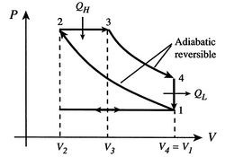
P-V Diagram for idealized Diesel cycle.
Efficiency of the Diesel Cycle
Because the process \(1 \rightarrow 2\) and \(3 \rightarrow 4\) are adiabatic, heat is not lost during those processes, so the efficiency can therefore be written in terms of the heat gained and lost, \(Q_H\) and \(Q_L\), as indicated on the diagram.
From the equation given above we can say that the heat gained \(Q_H\) is given in terms of specific heat and temperature by:
\begin{equation} Q_H = C_p (T_3 – T_2) \label{eq:q1} \end{equation}
We can likewise deduce the heat lost as \(Q=\int_{4 \rightarrow 1} C_V dT\) such that
\begin{equation} Q_L = C_V (T_1 – T_4) \label{eq:q2} \end{equation}
The thermal efficiency is defined as1 \(\eta={Q_H+Q_L \over Q_H}\), which we can express using \eqref{eq:q1} and \eqref{eq:q2} in the form of specific heats and temperatures \begin{equation} \eta=1+{C_V(T_1-T_4) \over C_p(T_3-T_2)} \label{eq:etaq1q2} \end{equation}
Using the ideal gas law \(PV=nRT\) where the \(n\)s and \(R\)s cancel, and the adiabatic index \(\gamma = {C_p \over C_V}\) we can further write
\[\eta = 1 + \gamma^{-1} {P_1 V_1 - P_4 V_4 \over P_3 V_3 - P_2 V_2}\]
From the diagram it can be seen that the volume V is the same in state 4 as in 1, i.e. \(V_4=V_1\). Likewise for pressure, \(P_3=P_2\). Therefore we can reduce our number of variables so that
\[\eta = 1 + \gamma^{-1} {V_1(P_1 - P_4) \over P_3(V_3-V_2)}\]
Dividing the fraction through by \(P_3V_1\):
\[\eta = 1+\gamma^{-1} {\frac{P_1}{P_3} - \frac{P_4}{P_3} \over R_{31} - R_{21}}\]
where \(R_{31} := \frac{V_3}{V_1}\) and \(R_{21} := \frac{V_2}{V_1}\).
For an adiabatic expansion, \(PV^{\gamma}\) is constant. Exploiting this fact, we can see from the diagram that the following relations hold:
\begin{eqnarray} \frac{P_1}{P_3}&=&\left( {V_2 \over V_1} \right)^{\gamma} &=& R_{21}^{\gamma} \nonumber \\ \frac{P_4}{P_3}&=&\left( {V_3 \over V_1} \right)^{\gamma} &=& R_{31}^{\gamma} \nonumber \end{eqnarray}
Finally, putting these back in and playing with minus signs:
\[ \eta = 1 - \gamma^{-1} {R_{31}^{\gamma} - R_{21}^{\gamma} \over R_{31} - R_{21}} ; \blacksquare \]
-
See MIT’s brief page about the Diesel cycle. It’s also whence I nicked my diagram. ↩︎